• What’s up with the noise!

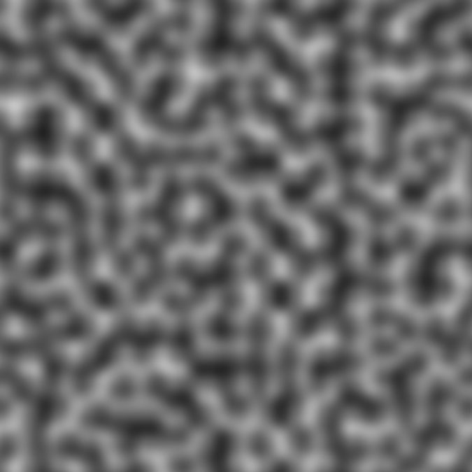
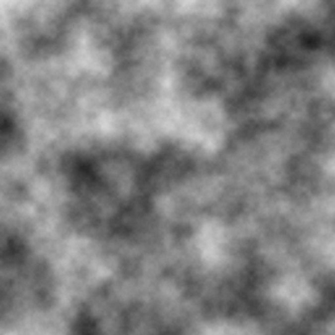
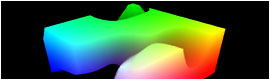
Noise can be thought of as an error imposed over a signal or measurement of data.

In Computer Graphics (CG), noise can help simulate naturally occurring phenomena that would be very difficult to generate otherwise.

Usually, random noise is no good, as Einstein said "God does not play dice with the universe". Otherwise, we would have tropical trees scattered around polar glaciers.

This is why researchers seek ways to produce noises, that generate coherent values with parameters that make them highly controllable, while remaining "random" to the human eye. They fall into a category called "Procedural Generation".

One of the most famous noises is the Perlin Noise, created by Ken Perlin, to produce organic textures for the movie "Tron", in 1982. The film received an Academy Award for Technical Achievement (14 years later).

Nowadays, noises are widely used to create all sorts of special effects: clouds, fire, organic textures, terrain generation, object scattering and real-Time mesh wreckage in game physics engines.

// This is simple Perlin Noise

// This is a fractal Perlin Noise, where many scaled versions are applied on top of each other:

• Voronoi Diagram and Worley Noise

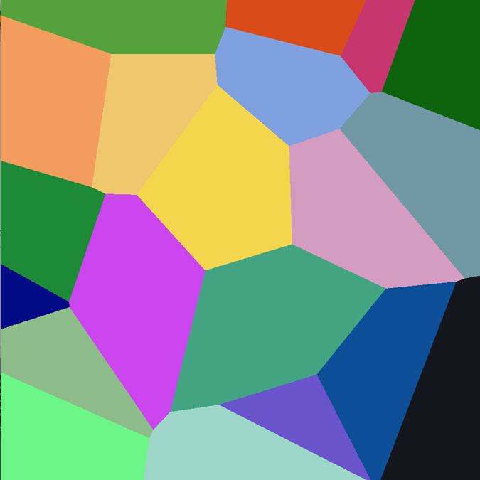
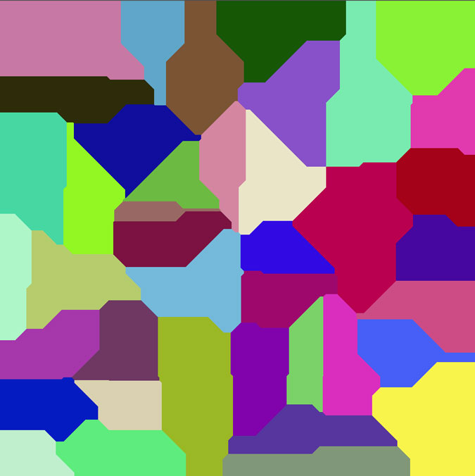
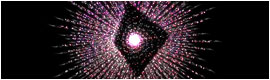
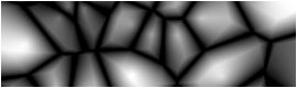
Used in optimization, the Voronoi diagram can also be used to produce textures, and it’s also widely used in CG.

Let’s take a look at the algorithm implemented in a 2D plane in a screen:

1. Generate random points across the area. These are the "feature points", and they have properties, like color, in our case.
2. For each of the pixels in the area:
   2.1 – Measure the distance to each feature points.
   2.2 - Recognize which feature point is closer: that is find the minimum distance.
   2.3 - Inherit/transfer properties of the nearest feature point to the point/pixel

That’s it!

This means that, if the pixel inherits the color of the feature point, we will end up with a vitraux-like plane, where each colored area represents all the pixels nearest to a certain feature point of the same color.

// Voronoi Diagram

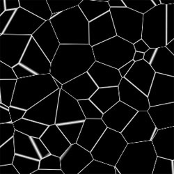
// Voronoi Diagram with Area Edges

But it does not end here: we can tweak some parts of the algorithm to come up with totally different patterns.

For example:
What if we change the way we measure the distance in step 2.1?

The first image measures distances using the euclidean distance.
If A=(xa,ya) and B=(xb, yb) are 2-dimensional points, the euclidean distance between them is

d(A,B)=sqrt((xa-xb)²+(ya-yb)²)

But in CG you could use other distances, for example: Manhattan, Chebyshev, and Minkowski distances.
Let’s take a look at just one of them: Manhattan distance between the points A and B would be

d(A,B)= abs(xa-xb) + abs(ya-yb)

This distance is also called TaxiCab distance, since it would be the shortest distance that one could travel in a city, where it is not possible to move diagonally.

// Voronoi Diagram with Manhattan Distance

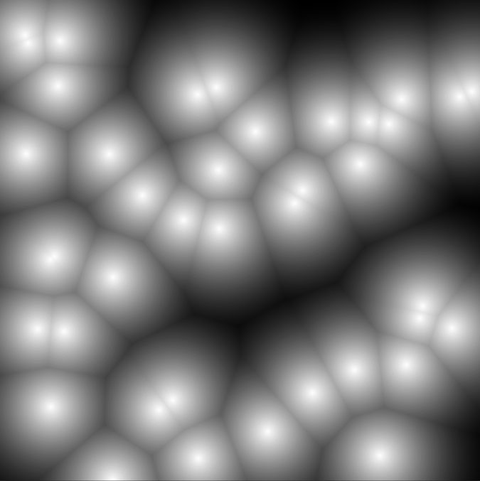
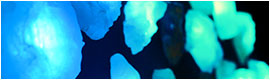
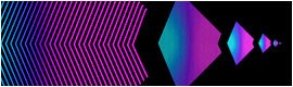
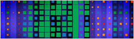
Usually, in CG, if we want to create a texture to control something other than the color of an object, we would create a grayscale image, because it represents an easy-to-handle 1-dimensional gradient. This means working with 1 range/scale of values at a time.

Different types of grayscale images can be generated by playing around with the Voronoi algorithm.

So, instead of inheriting the color, the pixel becomes a grayscale value, which is linearly interpolated between 0 and a specified maximum range.

// Worley Noise (Distance: Linear Interpolation to closest Feature Point)

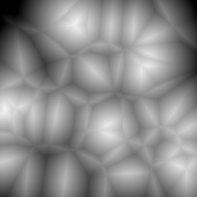
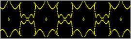
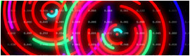
Welcome to the Worley family of noises, where what matters is the type of Interpolation and the Feature Selection.

What does this mean?
You can interpolate the distance from the pixel to the feature in whatever way you like, for example:

Linear: sqrt(a²+b²)
Linear Squared: a² + b²
Quadratic: (a² + a*b + b²)

Or any other operation…

And what does Feature Selection mean?

All these distances are calculated from the pixel position towards the closest Feature Point. There are variations, called "F values", which take into account the distance to the second closest Feature Point, or the third, or the nth.

// Worley Noise (Distance: Linear Interpolation to Second closest Feature Point)

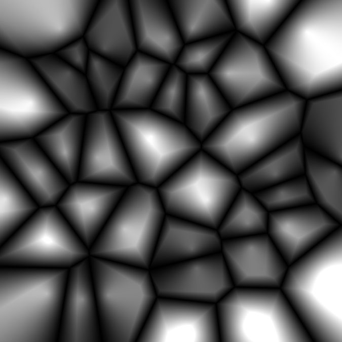
Other variations include operations between F values

The following is F2 minus F1:

// Worley Noise (Distance: Linear Interpolation to the difference between the second and the first closest Feature Point)

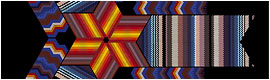
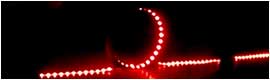
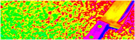
As you can see, a lot of these noises can be use to create textures of all sorts, such as leather, animal skin or scales, some plastics, or clouds, and a lot more with some creativity and playing around with the parameters.

During "La Semana de la Matemática" ("Math Week"), an event organized by the Buenos Aires University, Julia Picabea and I had the opportunity to make a presentation about Noise, "Procedural Generation of nth Dimensional Noise" specifically.

We prepared a small talk oriented towards the procedural generation of textures and maps used in 3D Animation, film and videoGame industry. This approach, we believe, softens the hard-algorithm impact that might scare people away, by providing a known frame.

We started out by explaining how noise is, showed an example of a procedure using Voronoi Diagrams, and finally did a realTime demonstration inside a 3d Modelling Application, of how to create a realistic stone, from a simple cube, using nothing but procedural noises. This is what we learned in the process.

• Check out some examples in this interactive web applet we created:
  Procedural Noises Examples

Also, take a look at the Poster we presented, where you can find some of the stuff explained here, plus a walkthrough of how to create a 3D Stone, in a 3D modelling application, starting from just a simple cube, using nothing but noises. It’s quite interesting.

// Julia Picabea and I presenting noise in a 3D landscape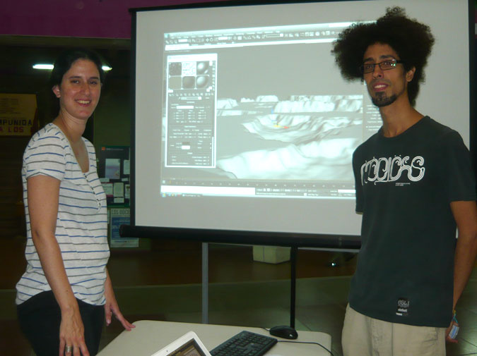

// Explaining the rendering of a Worley Noise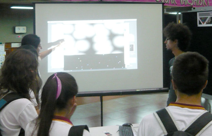